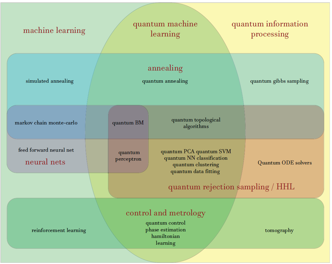
Quantum Machine Learning
Classical ML vs Quantum ML vs Hybrid ML
Quantum Kernel Methods for Perception & Decision
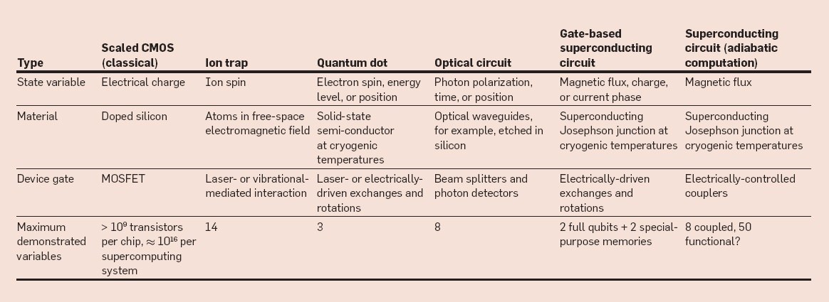
NISQ (Noisy Intermediate-Scale Quantum)
All quantum models in this work are designed for NISQ hardware, employing shallow variational circuits and hybrid optimization to mitigate decoherence and gate noise.
Let us write the most basic Quantum Program
pip3 install pennylane
import pennylane as qml
import numpy as np
# Create a quantum device with 1 qubit
dev = qml.device("default.qubit", wires=1)
@qml.qnode(dev)
def quantum_hello():
    qml.Hadamard(wires=0)        # Put qubit into superposition
    return qml.probs(wires=0)    # Measure probabilities

print(quantum_hello())
If you run the above snippet , you would see something like
[0.5 0.5]
Basically this is
Encode → Entangle → Measure → Optimize
Now that we have a small QC module , lets extend it
import pennylane as qml
from pennylane import numpy as np

dev = qml.device("default.qubit", wires=1)


@qml.qnode(dev)
def vqc(theta):
    qml.RY(theta, wires=0)     # trainable rotation
    return qml.expval(qml.PauliZ(0))

theta = 0.3
print(vqc(theta))

def loss(theta):
    return (vqc(theta) - 1.0) ** 2

opt = qml.GradientDescentOptimizer(stepsize=0.1)

theta = np.array(0.0, requires_grad=True)

for step in range(30):
    theta = opt.step(loss, theta)
    if step % 5 == 0:
        print(f"Step {step} | theta = {theta:.3f} | loss = {loss(theta):.4f}")
$
0.9553364891256059
Step 0 | theta = 0.000 | loss = 0.0000
Step 5 | theta = 0.000 | loss = 0.0000
Step 10 | theta = 0.000 | loss = 0.0000
Step 15 | theta = 0.000 | loss = 0.0000
Step 20 | theta = 0.000 | loss = 0.0000
Step 25 | theta = 0.000 | loss = 0.0000
🧠 What this means physically
- theta = trainable parameter
- Circuit prepares a quantum state
- Measurement returns ⟨Z⟩ expectation
- This is your model output
This is exactly like a neuron:
input → weight → activation
Every QML model is just:
[VQC] + [Classical Optimizer]
Now let us build a quantum neuron
The VQC now extended to behave like a quantum neuron
x → encode(x) → trainable circuit → output
import pennylane as qml
from pennylane import numpy as np

dev = qml.device("default.qubit", wires=1)

@qml.qnode(dev)
def vqc(x, theta):
    # 1️⃣ Encode classical input
    qml.RY(x, wires=0)

    # 2️⃣ Trainable rotation
    qml.RY(theta, wires=0)

    # 3️⃣ Readout
    return qml.expval(qml.PauliZ(0))

x = 0.5        # classical input feature
theta = 0.3   # trainable parameter

print(vqc(x, theta))

def loss(theta, x):
    return (vqc(x, theta) - 1.0) ** 2


opt = qml.GradientDescentOptimizer(stepsize=0.1)
theta = np.array(0.0, requires_grad=True)

x = 0.8  # fixed training input

for step in range(30):
    theta = opt.step(lambda t: loss(t, x), theta)

    if step % 5 == 0:
        print(
            f"Step {step} | "
            f"theta = {theta:.3f} | "
            f"output = {vqc(x, theta):.4f}"
        )
0.6967067093471653
Step 0 | theta = -0.044 | output = 0.7273
Step 5 | theta = -0.191 | output = 0.8200
Step 10 | theta = -0.277 | output = 0.8664
Step 15 | theta = -0.335 | output = 0.8939
Step 20 | theta = -0.378 | output = 0.9122
Step 25 | theta = -0.411 | output = 0.9251
Now let us add a quantumn entanglement node
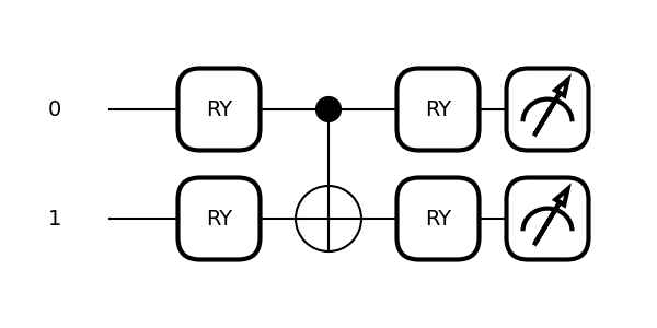
Let us go from
| 0⟩ ── RY(x) ── RY(θ) ── ⟨Z⟩ |
To
|0⟩ ── RY(x₁) ──●── RY(θ₁) ── ⟨Z⟩ │ |0⟩ ── RY(x₂) ──X── RY(θ₂) ── ⟨Z⟩
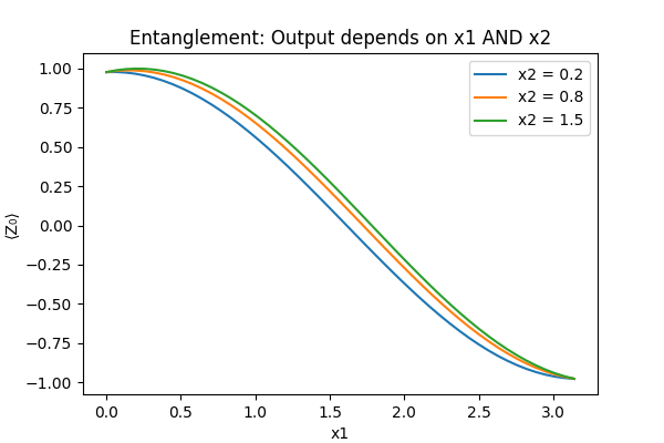
So that we achieve
✔ Correlated features ✔ Non-linear decision boundaries ✔ True quantum behavior
Probably confusing , my mind is stil tuned to the classical way of thinking , so let us take a analogy
x1 = distance x2 = relative speed risk = f(x1) + f(x2)
The risk in a real world driving would be a combination of distance AND speed together
risk ≠ f(x1) + f(x2) risk = f(x1, x2)
So without entanglement
Qubit 0 depends only on x1 Qubit 1 depends only on x2
With entanglement
Qubit 0 state depends on x1 AND x2 Qubit 1 state depends on x1 AND x2
import pennylane as qml
from pennylane import numpy as np

dev = qml.device("default.qubit", wires=2)

@qml.qnode(dev)
def entangled_vqc(x, theta):
    # x: 2-dim classical input
    # theta: 2 trainable params

    # 1️⃣ Encode classical features
    qml.RY(x[0], wires=0)
    qml.RY(x[1], wires=1)

    # 2️⃣ Entanglement
    qml.CNOT(wires=[0, 1])

    # 3️⃣ Trainable rotations
    qml.RY(theta[0], wires=0)
    qml.RY(theta[1], wires=1)

    # 4️⃣ Readout
    return (
        qml.expval(qml.PauliZ(0)),
        qml.expval(qml.PauliZ(1))
    )


x = np.array([0.6, 0.2])
theta = np.array([0.1, 0.1])

print(entangled_vqc(x, theta))


def loss(theta, x):
    z0, z1 = entangled_vqc(x, theta)
    return (z0 - 1.0) ** 2 + (z1 - 1.0) ** 2


opt = qml.GradientDescentOptimizer(stepsize=0.1)
theta = np.array([0.0, 0.0], requires_grad=True)

x = np.array([0.8, 0.3])

for step in range(30):
    theta = opt.step(lambda t: loss(t, x), theta)

    if step % 5 == 0:
        z0, z1 = entangled_vqc(x, theta)
        print(
            f"Step {step} | "
            f"theta = {theta} | "
            f"Z = ({z0:.3f}, {z1:.3f})"
        )
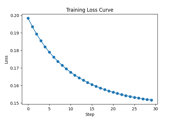
Step 0 | theta = [-0.01285922 -0.01976502] | Z = (0.699, 0.671)
Step 5 | theta = [-0.06818813 -0.10245817] | Z = (0.710, 0.692)
Step 10 | theta = [-0.1116638  -0.16518783] | Z = (0.716, 0.705)
Step 15 | theta = [-0.14628707 -0.21403244] | Z = (0.720, 0.713)
Step 20 | theta = [-0.17410229 -0.25270375] | Z = (0.723, 0.718)
Step 25 | theta = [-0.1965766  -0.28365224] | Z = (0.725, 0.722)
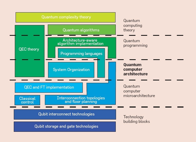
End-to-End Quantum Machine Learning Architecture