Text Processing
Different NLP and text processing techniques
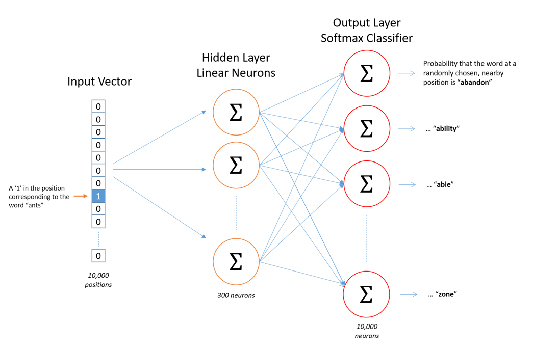
Word to Vec Techniques
There are two common Word2Vec models for learning word embeddings from preprocessed text data:
- Continuous Bag of Words (CBOW): This model predicts the context words from the target word in a given window of text.
- Skip-Gram (SKI gram): The Skip-Gram model works inversely by predicting the target word from the surrounding context words.
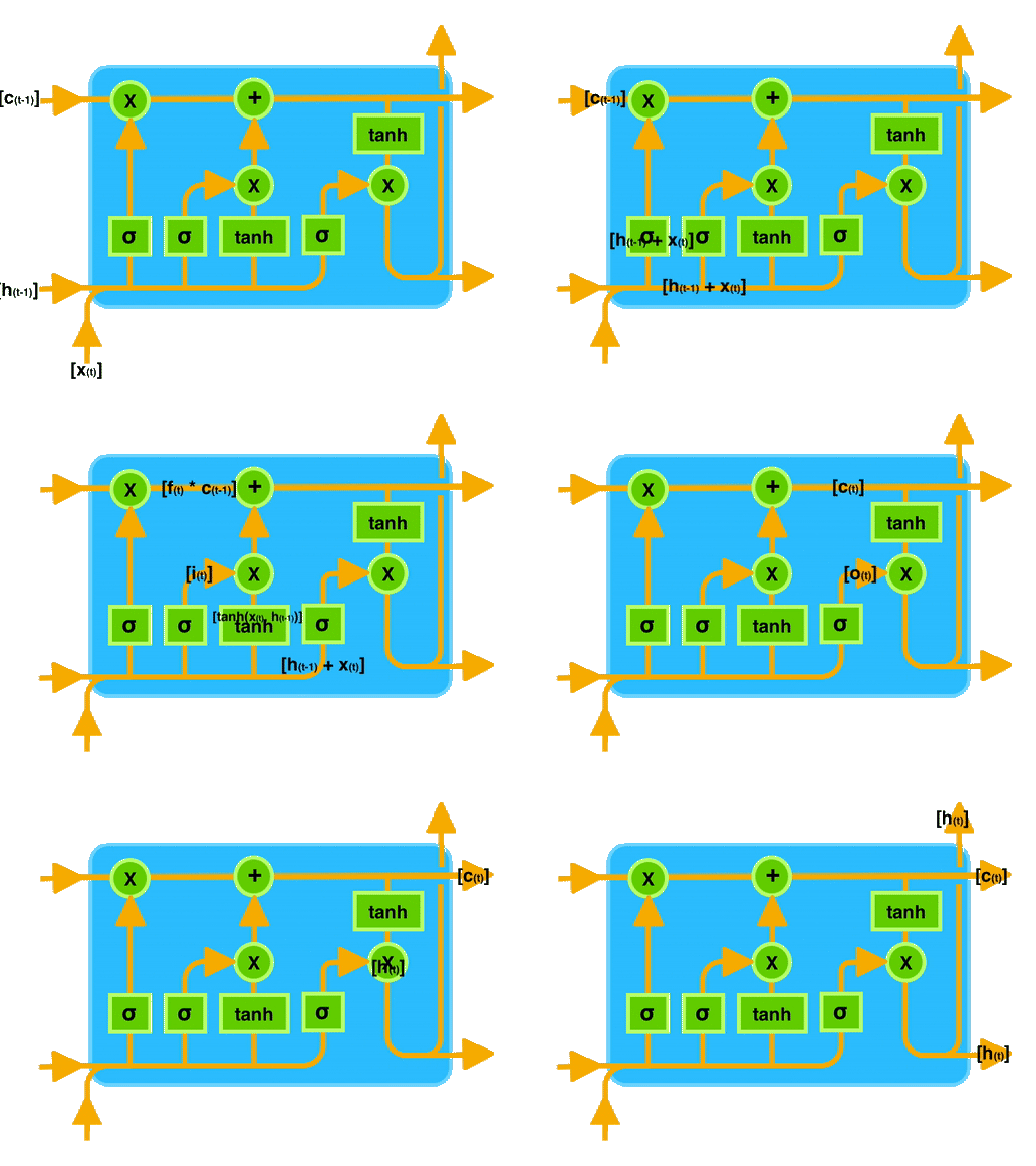
LSTM (Long Short-Term Memory)
Recurrent Neural Networks (RNNs) are designed for sequential data, but they struggle with long-term dependencies due to the vanishing gradient problem. LSTM is a more advanced type of RNN, designed specifically to overcome this issue by using memory cells and gates to store long-term information.
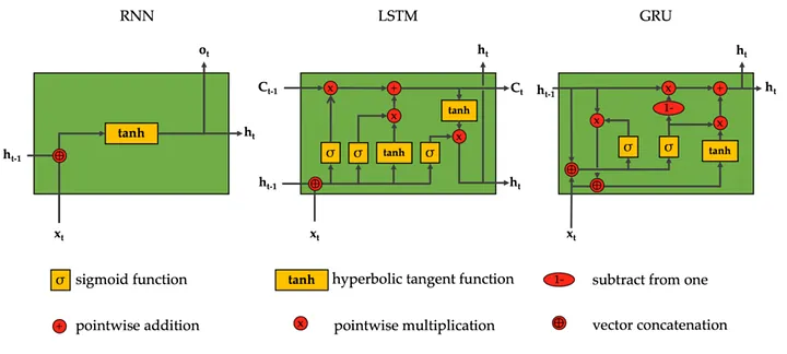
Architecture Comparison:
- RNN: Simple recurrent connections, which can struggle with long-term dependencies.
- LSTM: Complex architecture with memory cells and three gates (input, output, forget) that help capture long-term dependencies.
- GRU (Gated Recurrent Unit): A simplified version of LSTM, using two gates, often more efficient in terms of training time.
Learning Capabilities:
- RNN: Best for short-term dependencies.
- LSTM: Superior for capturing long-term dependencies in complex sequences.
- GRU: Similar to LSTM but faster and with a slightly simplified structure.
Training Complexity:
- RNN: Easier to implement but less effective for long-term dependencies.
- LSTM: More complex and computationally intensive, requiring careful tuning.
- GRU: Simpler and faster to train, often achieving similar performance to LSTM.
Transformers
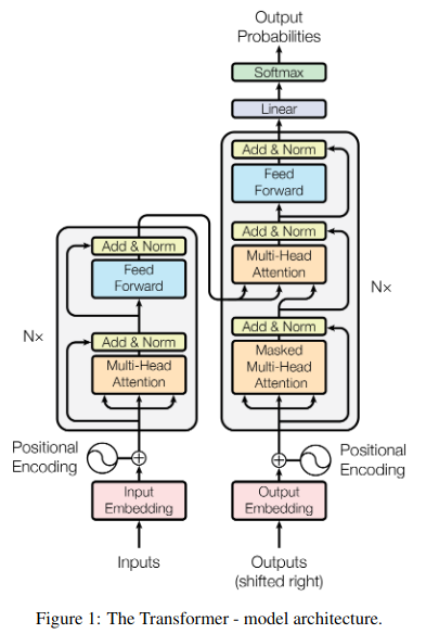
The Transformer model revolutionized NLP with its “Attention Is All You Need” approach, focusing solely on attention mechanisms, rather than using recurrent layers. This has led to faster processing and better performance for large datasets.
Key Benefits of Transformers:
- Parallelization: Unlike RNNs, Transformers do not require sequential processing, allowing for faster computation.
- Self-Attention: Each word in the sequence is able to attend to all other words simultaneously, helping capture dependencies more efficiently.
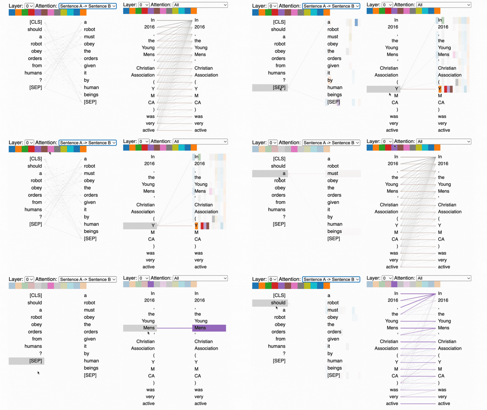
BERT (Bidirectional Encoder Representations from Transformers)
BERT is a pre-trained transformer model designed to understand the context of words in relation to all other words in a sentence, making it bidirectional. This is a breakthrough for tasks like question answering and language inference.

Exploring NLP Techniques: Word Embeddings and More
Natural Language Processing (NLP) encompasses a wide range of techniques to transform and understand human language. In this post, we’ll walk through some key NLP concepts, from data pre-processing to advanced word embedding techniques like CBOW, Skip-Gram, and LSA. These tools are foundational for many applications in text classification, sentiment analysis, and language modeling.
Preprocessing Text Data
Before diving into NLP models, preprocessing text data is essential for making it more suitable for analysis. The following steps outline common preprocessing techniques:
1. Tokenization
Tokenization is the process of splitting text into smaller components such as words or sentences. For example, the sentence “Mohan does not like reading” is split into tokens: ['Mohan', 'does', 'not', 'like', 'reading'].
2. Stopword Removal
Stopwords are common words (like “does”, “not”, “the”) that usually don’t carry significant meaning in text analysis. Removing them helps reduce noise in the data. After stopword removal, the sentence could look like: ['Mohan', 'like', 'reading'].
3. Lemmatization and Stemming
Both lemmatization and stemming reduce words to their root form. Lemmatization ensures that words like “running” become “run,” while stemming might reduce it to “run” as well but in a more mechanical fashion (e.g., “running” → “run”).
After applying these steps, text data is more structured and ready for feature extraction.
Representing Text Data: Binary, TF, and TF-IDF
Once the data is preprocessed, it’s time to convert it into a numerical format. Let’s explore common methods:
1. Binary Representation
In this method, we simply mark the presence or absence of each word in the document. If a word appears in the sentence, we assign it a 1; otherwise, it’s a 0.
For example:
2. Term Frequency (TF)
TF counts the number of times a word appears in a document. Words that appear more frequently are weighted higher. For example:
- Sentence: “Mohan likes reading and reading is fun.”
- TF for “reading”: 2 (since it appears twice).
3. TF-IDF (Term Frequency - Inverse Document Frequency)
TF-IDF adjusts the frequency of terms by considering their importance across all documents. It penalizes terms that appear frequently across many documents, as they are less informative. The formula for TF-IDF is: [ \text{TF-IDF}(t) = \text{TF}(t) \times \log\left(\frac{N}{df(t)}\right) ] where (N) is the total number of documents and (df(t)) is the number of documents containing the term (t).
Word Embedding Techniques
Word embeddings help convert words into dense vectors, allowing machine learning models to capture semantic meaning. Let’s explore a few common methods:
1. One-Hot Encoding
One-hot encoding is the simplest form of word embedding. Each word is represented as a vector, where the index corresponding to the word is set to 1, and all other indices are set to 0. While simple, this method doesn’t capture semantic relationships between words (e.g., “dog” and “cat” would have no relationship).
2. Continuous Bag of Words (CBOW) and Skip-Gram
CBOW and Skip-Gram are two models in Word2Vec that use neural networks to learn word embeddings based on their context:
- CBOW: Predicts the target word based on its surrounding context words. If we consider the sentence “Mohan reads well” with a context window of size 1, CBOW would predict “reads” using “Mohan” and “well”.
- Skip-Gram: The inverse of CBOW, where the target word predicts its context. In the same example, “reads” would predict “Mohan” and “well.”
Both models are designed to capture semantic meanings based on word co-occurrence patterns.
3. Latent Semantic Analysis (LSA)
LSA uses Singular Value Decomposition (SVD) to reduce a Term-Document matrix into a lower-dimensional space. It captures latent semantic structures and represents words in a continuous vector space. While effective, LSA doesn’t handle large datasets as efficiently as models like Word2Vec or BERT.
Embedding Generation for Text Data
Once trained, these models can generate embeddings for both training and test data. For instance, after training CBOW or Skip-Gram models on a corpus, each word is represented as a vector in the learned embedding space. Similarly, LSA applies SVD to produce a lower-dimensional representation of words and sentences.
Aggregating Embeddings
To create embeddings for entire sentences, one can aggregate word embeddings. A common method is averaging the embeddings of all words in the sentence, which provides a single vector representation for the entire sentence or document.
Augmenting Training Data
Data augmentation is a valuable technique to increase the diversity of the training data without collecting new data. For example, paraphrasing can be used to generate new training examples by altering sentence structures without changing their meaning.
Sentiment Analysis with Neural Networks
In this section, we will cover how to implement a sentiment analysis model using deep learning and word embeddings. The goal is to classify text data into sentiment categories such as positive, negative, or neutral.
1. Data Preprocessing
We begin by tokenizing the text, removing stopwords, and applying lemmatization.
import nltk
from nltk.tokenize import word_tokenize
from nltk.corpus import stopwords
from nltk.stem import WordNetLemmatizer

# Download necessary resources
nltk.download('punkt')
nltk.download('stopwords')
nltk.download('wordnet')

# Initialize lemmatizer
lemmatizer = WordNetLemmatizer()

# Sample sentence
sentence = "I love machine learning, it's so fascinating!"

# Tokenization
tokens = word_tokenize(sentence)

# Stopword removal
stop_words = set(stopwords.words('english'))
tokens = [word for word in tokens if word.lower() not in stop_words]

# Lemmatization
tokens = [lemmatizer.lemmatize(word) for word in tokens]
print(tokens)
import numpy as np
import tensorflow as tf
from tensorflow.keras.models import Sequential
from tensorflow.keras.layers import Dense, Embedding, LSTM, SpatialDropout1D
from tensorflow.keras.preprocessing.sequence import pad_sequences

# Assuming X_train, X_test, y_train, y_test are prepared data
model = Sequential()
model.add(Embedding(input_dim=5000, output_dim=128, input_length=X_train.shape[1]))
model.add(SpatialDropout1D(0.2))
model.add(LSTM(100, dropout=0.2, recurrent_dropout=0.2))
model.add(Dense(1, activation='sigmoid'))

model.compile(loss='binary_crossentropy', optimizer='adam', metrics=['accuracy'])

# Train the model
model.fit(X_train, y_train, epochs=10, batch_size=32, validation_split=0.2)
from sklearn.metrics import accuracy_score, precision_score, recall_score, f1_score

# Predict sentiment for test data
y_pred = model.predict(X_test)

# Convert predictions to binary values
y_pred_binary = [1 if pred > 0.5 else 0 for pred in y_pred]

# Evaluate the model
accuracy = accuracy_score(y_test, y_pred_binary)
precision = precision_score(y_test, y_pred_binary)
recall = recall_score(y_test, y_pred_binary)
f1 = f1_score(y_test, y_pred_binary)

print(f"Accuracy: {accuracy}")
print(f"Precision: {precision}")
print(f"Recall: {recall}")
print(f"F1 Score: {f1}")
This project highlights the use of preprocessing techniques and word embeddings (CBOW and Skip-Gram) to perform sentiment analysis. The neural network built using Keras demonstrated how to classify sentiments in text data, and the evaluation metrics showed the model’s performance.
By leveraging the power of word embeddings and deep learning, we can tackle a wide range of natural language processing tasks, including sentiment analysis, text classification, and language translation.
CLASS NOTES
RNN (2017)
LSTM
- Very unstable
- Very hard to train
Attention
- Information shared beteween Encoder and Decoder
- Positional encodings were added using hand crafted features like sinosodila functions
Transformer (2018)
- Initial goal for an architecture Encoder Decoder
- Get rid of recurrence
- replace with self attention
- Sequence to sequence models became easy
- Preserves sentence structures .
- Various stacks of Encoders and Decoders
- Self Attention feed forward
Self Attention
- Self attention is the key layer in a transformer stack
- Get 3 vectors for each embedding Query , Key and Value
- Scale , MatMul , SoftMax
- Finaly outputs Scores(because we do a Dot product )
- A.B = A B cos(theta)
- Will give distance
- AxB = A B sin(theta)
- will give direction
- Tranfformers have Multiple heads and Attention
- LLMs are trained on large datasets
- Positional Encoding , how this works
- Its notghin but a vector of the same length .
- sin and cosine embedding
-
Self Attention Add , normalization layer , Earliest problem was diminishing gradient , float numbers were becoming realy small , working with decimal numbers is always a problem , gradient back propagration was always ending up as zero . Residual connection was doing it at every layer Added layer normalization , its different from batch normalizaiton , it learns two parameters . What it does it , it learnds means and adds a huge number of parameters . We can switch off these layers in fine tuning . Sometimes tries to remove these laers .
- What happens in a Decoders?
- Masked multihead self attention
- Multi headed attention layer over encoder output
- Position wise feed forward layer
- Each sublayer has a residuals connection and is normalized LayerNorma(x + Sublayer(x))
| Architecture | Inventors | Introduction Date | Pros | Cons | Architecture Diagram |
|---|---|---|---|---|---|
| Recurrent Neural Networks (RNNs) | John Hopfield (1982) | 1980s | - Suitable for sequential data processing. - Captures temporal dynamics. | - Suffers from vanishing and exploding gradient problems. - Struggles with long-term dependencies. |  |
| Long Short-Term Memory (LSTM) | Sepp Hochreiter and Jürgen Schmidhuber | 1997 | - Addresses vanishing gradient problem. - Capable of learning long-term dependencies. | - Computationally intensive. - Complex architecture. |  |
| Attention Mechanism | Dzmitry Bahdanau, Kyunghyun Cho, and Yoshua Bengio | 2014 | - Allows the model to focus on relevant parts of the input sequence. - Improves performance on tasks like machine translation. | - Increases computational complexity. - May require large amounts of data to train effectively. |  |
| Transformer | Ashish Vaswani, Noam Shazeer, Niki Parmar, Jakob Uszkoreit, Llion Jones, Aidan N. Gomez, Łukasz Kaiser, and Illia Polosukhin | 2017 | - Enables parallel processing of sequence data. - Captures long-range dependencies effectively. - Reduces training time compared to RNNs and LSTMs. | - Requires large datasets and computational resources. - May struggle with very long sequences due to fixed input size during training. |  |
Positional Encoding and Decoders in Transformers
Positional Encoding
-
Purpose: Adds information about the position of tokens in a sequence since Transformers lack inherent sequential understanding.
- Mechanism:
- Positional encoding is a vector of the same length as token embeddings.
- Encoded using sinusoidal functions:
- Formula: \(PE(pos, 2i) = \sin\left(\frac{pos}{10000^{\frac{2i}{d_{\text{model}}}}}\right)\) \(PE(pos, 2i+1) = \cos\left(\frac{pos}{10000^{\frac{2i}{d_{\text{model}}}}}\right)\) Where:
- ( pos ): Position of the token in the sequence.
- ( i ): Dimension index.
- ( d_{\text{model}} ): Dimensionality of embeddings.
- Formula: \(PE(pos, 2i) = \sin\left(\frac{pos}{10000^{\frac{2i}{d_{\text{model}}}}}\right)\) \(PE(pos, 2i+1) = \cos\left(\frac{pos}{10000^{\frac{2i}{d_{\text{model}}}}}\right)\) Where:
- Smooth encoding allows the model to infer relative positions.
- Integration: Added to token embeddings before passing to the self-attention layers.
Self-Attention with Residual Connections
- Gradient Vanishing Problem:
- Small gradients caused ineffective learning in earlier deep networks, especially with long sequences.
- Residual Connections:
- Skip connections pass input directly to the layer output: \(y = \text{LayerNorm}(x + \text{Sublayer}(x))\)
- Helps stabilize gradient flow and improves training.
- Layer Normalization:
- Normalizes across features of a single data point instead of batch-wise.
- Key Differences from Batch Normalization:
- Operates on individual samples, not batches.
- Learns mean and variance parameters for flexibility.
- Can be disabled during fine-tuning to reduce parameter overhead.
Decoders in Transformers
- Functionality:
- Generates the output sequence token by token.
- Attends to encoder outputs and previously generated tokens.
- Components:
- Masked Multi-Head Self-Attention:
- Ensures causal masking by preventing attention to future tokens.
- Multi-Head Attention Layer over Encoder Outputs:
- Allows focusing on relevant encoder outputs for each token.
- Position-Wise Feed-Forward Layer:
- Applies fully connected layers to each position independently, enabling non-linear transformations.
- Masked Multi-Head Self-Attention:
- Residual Connections and Layer Normalization:
- Each sublayer includes:
- Residual connections to address gradient issues.
- Layer normalization for numerical stability and consistent learning.
- Each sublayer includes:
GPT, Codex, DALL-E, and Foundation Models
Overview Table
| Technology | Inventor | Date | Key Features | Applications | Pros | Cons |
|---|---|---|---|---|---|---|
| GPT (Generative Pre-trained Transformer) | OpenAI | 2018 (GPT-1), 2020 (GPT-3) | Based on the Transformer model (decoder-only architecture). Pretrained on large text datasets. Goal: AGI-like capabilities. | Chatbots, writing assistants, language modeling, code generation. | High-quality language generation, scalable for various tasks, pre-trained on vast data. | Lacks reasoning skills, expensive training, potential for generating harmful/biased content. |
| Codex | OpenAI | 2021 | Variant of GPT-3 tailored for code understanding and generation. Supports dozens of programming languages. | Code completion (e.g., GitHub Copilot), debugging, automation. | Accelerates software development, supports multi-language programming. | Limited reasoning about program logic, sometimes produces insecure code or incorrect outputs. |
| DALL-E | OpenAI | 2021 | Transformer-based model for text-to-image generation. Generates realistic and creative images from textual prompts. | Creative arts, marketing, advertising, image-based research. | High-quality and diverse image generation from natural language. | Struggles with complex prompts, risks of misuse (e.g., generating fake images). |
| Gemini (Google DeepMind) | Google DeepMind | 2023 | Multimodal AI system combining large-scale vision and language models. | Multimodal understanding (text, image), creative writing, analysis. | Powerful for multimodal tasks, advanced reasoning capabilities. | High computational cost, still developing. |
| Foundation Models | Multiple (OpenAI, Google, etc.) | 2020+ | Pretrained on multi-modal data: text, images, speech, tables, videos, point clouds. Fine-tunable for downstream tasks. Reinforcement Learning with Human Feedback (RLHF). | Healthcare, legal analysis, education, content creation, creative animation. | Generalized knowledge across modalities, transferable to specific domains, cost-effective for fine-tuning. | Expensive to pretrain, dependency on vast computational resources, ethical concerns regarding generated data. |
Foundational Models: Key Points
Applications:
- Text: Language models generate articles, emails, and assist with copywriting.
- Images: Creative animation, text-to-image systems (e.g., DALL-E).
- Speech: Text-to-speech systems, virtual assistants.
- Tables/Signals: Analyze and visualize structured data (e.g., Excel automation).
- Healthcare: Aid in diagnosing diseases, drug discovery.
- Education: Generate educational content, assist with personalized learning.
Challenges:
- Ethical Concerns: Unpaid human input used for training; concerns about data ownership.
- Accessibility: Expensive to train and deploy; limited to organizations with significant resources.
- Bias and Fairness: Models may reflect biases present in the training data.
Technical Explanations
Reinforcement Learning with Human Feedback (RLHF)
- Combines human feedback with reinforcement learning to fine-tune model outputs.
- Formula: \(\text{Reward Model: } R(x, y) = \sum_i \alpha_i \cdot f_i(x, y)\) Where:
- ( x ): Input prompt.
- ( y ): Model output.
- ( f_i ): Features or metrics defined by human evaluators.
- ( \alpha_i ): Weights for each metric.
Transfer Learning in Foundation Models
- Transfer learning involves pretraining on a large dataset and fine-tuning for specific tasks.
- Formula: \(\text{Fine-Tuned Loss: } L = L_{\text{task}} + \lambda \cdot L_{\text{pretrain}}\) Where:
- ( L_{\text{task}} ): Loss specific to the downstream task.
- ( L_{\text{pretrain}} ): Regularization term from the pretrained model.
- ( \lambda ): Weight balancing task-specific and pretrained losses.
Architecture Diagram
Below is a simplified architecture for GPT and Foundation Models:
```plaintext Input Sequence ↓ Token Embedding ↓ Positional Encoding ↓ Multi-Head Attention ↓ Feed-Forward ↓ Residual Add ↓ Layer Normalization ↓ Final Output (Token Prediction, Text, Image, etc.)